AGO-I: A real-time consumer intelligent guidance system based on IoT and multi-tasking user portrait

P.S. To protect code ownership and copyright, the code in this article may be simplified, hidden, and frequently use sample data, but this does not hinder the understanding of the core ideas.

Summary

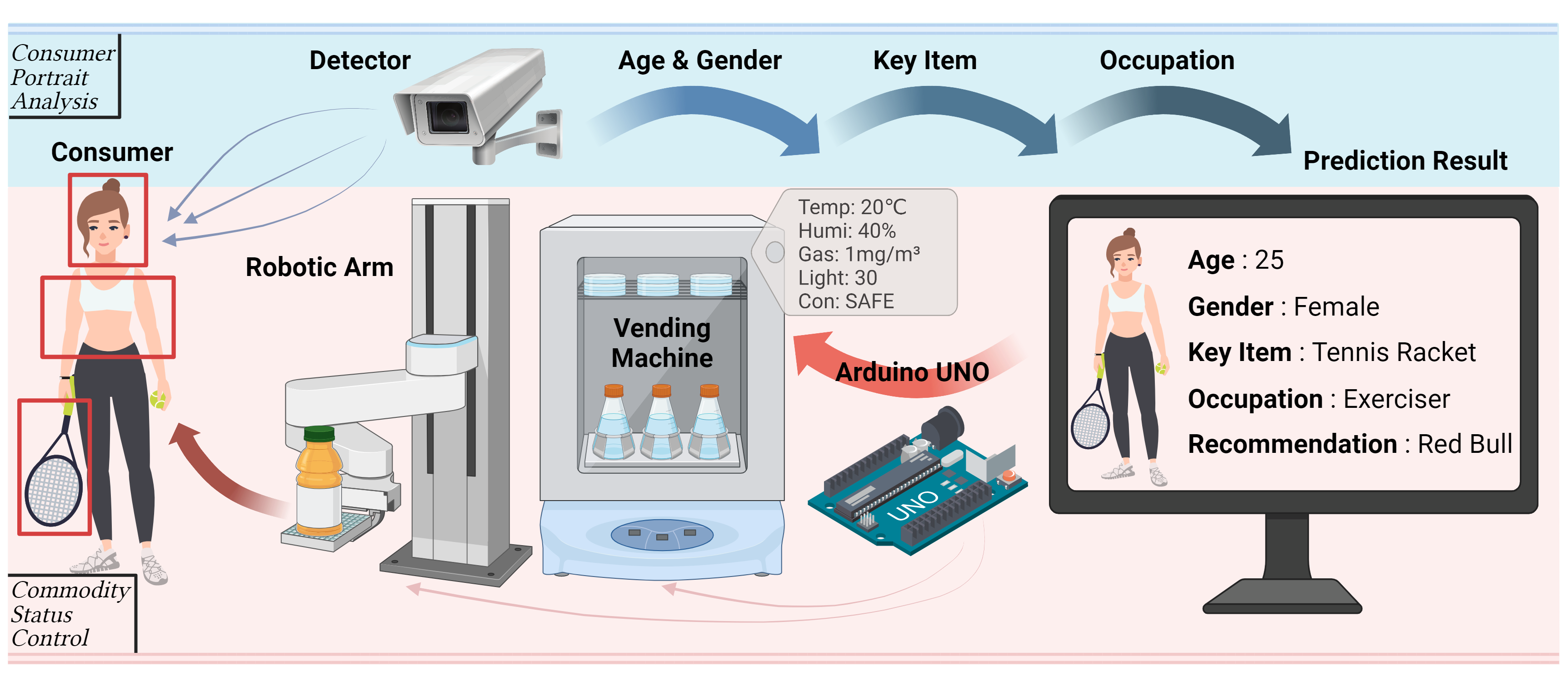
In the architecture of Society 5.0 actively promoted in Japan, the innovative retail industry is an essential component of the smart city, driving the high integration of network and physical space in the consumer industry. However, the AI facilities in various small and medium-sized stores in Japan are still at the level of some basic interactive applications. In order to improve the user’s consumption experience and effectively promote the intelligence, customization and scientific management of the shopping system, we have designed a consumer intelligent guidance system based on deep learning and IoT technology. The system has two branches: 1. A high-granularity user profiling analysis framework; 2. A low-cost product management kit. Through this system, we can efficiently and accurately predict the age, gender, occupation and current physical state of consumers in real-time without infringing on personal privacy. At the same time, it can unify the management of store merchandise and cooperate with the user analysis framework at the physical level to achieve intelligent product recommendations. In order to train a high-accuracy occupational classification model, we manually constructed a dataset containing four common occupations: JPOCC. After experimentation, our classification model has achieved excellent results in various indicators, and its training cost is relatively low.

1. System Architecture

1.1 Consumer Portrait Construction

1.1.1 Age and Gender Classification

Overview

• Introduction to the importance of age and gender classification in consumer analysis: Age and gender classification play a vital role in consumer analysis. By understanding the demographic details of customers, businesses can tailor their marketing strategies, product offerings, and services to meet the specific needs of different age groups and genders. This not only enhances customer satisfaction but also drives sales and loyalty.
• Brief description of the CaffeNet model used for classification: CaffeNet, a variant of the AlexNet architecture, is widely used for image classification tasks. In our case, we use it for age and gender classification. This model is pre-trained on a large dataset, allowing us to leverage its learned features for our specific application without needing an extensive training phase.

Implementation Details

• Description of the model architecture and key parameters: The architecture of the CaffeNet model includes multiple convolutional layers for feature extraction, followed by fully connected layers for classification. Key parameters include the input size of 227x227 pixels and specific mean values for image normalization.
• Steps for loading and using pre-trained models for face detection, age prediction, and gender prediction: Let’s dive into the code to see how we can load and use these pre-trained models.

First, we start with some essential imports and define a function to highlight detected faces in the input frame. This part of the work is inspired by smahesh29 on GitHub.

import cv2
import argparse

def highlightFace(net, frame, conf_threshold=0.7):
    frameOpencvDnn = frame.copy()
    frameHeight = frameOpencvDnn.shape[0]
    frameWidth = frameOpencvDnn.shape[1]
    blob = cv2.dnn.blobFromImage(frameOpencvDnn, 1.0, (300, 300), [104, 117, 123], True, False)

    net.setInput(blob)
    detections = net.forward()
    faceBoxes = []
    for i in range(detections.shape[2]):
        confidence = detections[0, 0, i, 2]
        if confidence > conf_threshold:
            x1 = int(detections[0, 0, i, 3] * frameWidth)
            y1 = int(detections[0, 0, i, 4] * frameHeight)
            x2 = int(detections[0, 0, i, 5] * frameWidth)
            y2 = int(detections[0, 0, i, 6] * frameHeight)
            faceBoxes.append([x1, y1, x2, y2])
            cv2.rectangle(frameOpencvDnn, (x1, y1), (x2, y2), (0, 255, 0), int(round(frameHeight / 150)), 8)
    return frameOpencvDnn, faceBoxes

In this function, we create a blob from the input image, which is then fed into the face detection model. The model returns a set of detections, from which we extract the bounding boxes of faces with a confidence score above the specified threshold. We draw rectangles around these faces for visualization. Next, let’s load our pre-trained models for face detection, age prediction, and gender prediction:

parser = argparse.ArgumentParser()
parser.add_argument('--image')
args = parser.parse_args()

faceProto = "opencv_face_detector.pbtxt"
faceModel = "opencv_face_detector_uint8.pb"
ageProto = "age_deploy.prototxt"
ageModel = "age_net.caffemodel"
genderProto = "gender_deploy.prototxt"
genderModel = "gender_net.caffemodel"

MODEL_MEAN_VALUES = (78.4263377603, 87.7689143744, 114.895847746)
ageList = ['(0-2)', '(4-6)', '(8-12)', '(15-20)', '(25-32)', '(38-43)', '(48-53)', '(60-100)']
genderList = ['Male', 'Female']

faceNet = cv2.dnn.readNet(faceModel, faceProto)
ageNet = cv2.dnn.readNet(ageModel, ageProto)
genderNet = cv2.dnn.readNet(genderModel, genderProto)

Here, we define the file paths for the model configurations and weights. We also specify the mean values for image normalization and the labels for age and gender categories. Using cv2.dnn.readNet, we load the pre-trained models into our program. Now, we can process the input image or video feed to detect faces and predict their age and gender:

video = cv2.VideoCapture(args.image if args.image else 0)
padding = 20

while cv2.waitKey(1) < 0:
    hasFrame, frame = video.read()
    if not hasFrame:
        cv2.waitKey()
        break

    resultImg, faceBoxes = highlightFace(faceNet, frame)
    if not faceBoxes:
        print("No face detected")

    for faceBox in faceBoxes:
        face = frame[max(0, faceBox[1] - padding):min(faceBox[3] + padding, frame.shape[0] - 1),
        max(0, faceBox[0] - padding):min(faceBox[2] + padding, frame.shape[1] - 1)]

        blob = cv2.dnn.blobFromImage(face, 1.0, (227, 227), MODEL_MEAN_VALUES, swapRB=False)
        genderNet.setInput(blob)
        genderPreds = genderNet.forward()
        gender = genderList[genderPreds[0].argmax()]
        print(f'Gender: {gender}')

        ageNet.setInput(blob)
        agePreds = ageNet.forward()
        age = ageList[agePreds[0].argmax()]
        print(f'Age: {age[1:-1]} years')

        cv2.putText(resultImg, f'{gender}, {age}', (faceBox[0], faceBox[1] - 10), cv2.FONT_HERSHEY_SIMPLEX, 0.8, (0, 255, 255), 2, cv2.LINE_AA)
        cv2.imshow("Detecting age and gender", resultImg)

In this loop, we capture frames from the video or image input, detect faces, and then predict the gender and age for each detected face. The results are displayed on the image in real-time. With these steps, we can accurately classify the age and gender of consumers, providing valuable insights for personalized marketing strategies. The combination of face detection, gender prediction, and age prediction models allows for a robust consumer portrait construction, enhancing the overall consumer analysis process. This part of the implementation is inspired by smahesh29 on GitHub.

1.1.2 Key Item Identification

Overview

• Purpose of key item identification in understanding consumer activities: Identifying key items that consumers interact with can provide insights into their interests and activities. This is crucial for understanding consumer behavior, preferences, and needs. For instance, detecting sports equipment can indicate an interest in fitness, which can be leveraged for targeted marketing and personalized recommendations.
• Categories of items identified (e.g., sports equipment): The system is designed to identify a variety of key items such as sports equipment, electronic gadgets, fashion accessories, and more. These categories help in segmenting consumers based on their interests and activities.

Methodology

• Use of Faster R-CNN with ResNet-50 and FPN for object detection: Faster R-CNN (Region-based Convolutional Neural Networks) is a state-of-the-art object detection model. By integrating it with ResNet-50 (a deep residual network) and FPN (Feature Pyramid Network), we achieve high accuracy and efficiency in detecting and classifying key items.
• Steps involved in detecting and classifying key items:
  1. Model Loading: Load the pre-trained Faster R-CNN model with ResNet-50 and FPN.
  2. Image Preprocessing: Preprocess the input images to the required format.
  3. Object Detection: Use the model to detect and classify objects in the images.
  4. Result Visualization: Draw bounding boxes around detected objects and label them with their categories.

Let’s look at a code snippet to illustrate this process:

import torch
from torchvision import models, transforms
from PIL import Image
import matplotlib.pyplot as plt
import matplotlib.patches as patches

# Load the pre-trained Faster R-CNN model
model = models.detection.fasterrcnn_resnet50_fpn(pretrained=True)
model.eval()

# Define the image transformation
transform = transforms.Compose([
    transforms.ToTensor(),
])

def detect_objects(image_path):
    image = Image.open(image_path).convert("RGB")
    image_tensor = transform(image).unsqueeze(0)

    with torch.no_grad():
        predictions = model(image_tensor)

    return image, predictions

def display_results(image, predictions, threshold=0.5):
    plt.figure(figsize=(12, 8))
    plt.imshow(image)
    ax = plt.gca()

    for element in predictions[0]['boxes']:
        x1, y1, x2, y2 = element
        rect = patches.Rectangle((x1, y1), x2 - x1, y2 - y1, linewidth=2, edgecolor='r', facecolor='none')
        ax.add_patch(rect)

    plt.show()

# Example usage
image_path = 'path_to_image.jpg'
image, predictions = detect_objects(image_path)
display_results(image, predictions)

Explanation:

• Model Loading: We load the pre-trained Faster R-CNN model with ResNet-50 and FPN.
• Image Transformation: The input image is transformed into a tensor.
• Object Detection: The model predicts the bounding boxes and labels for objects in the image.
• Result Visualization: Bounding boxes are drawn around detected objects, and the results are displayed using Matplotlib.

This approach enables us to accurately detect and classify key items, providing valuable data for consumer activity analysis. By understanding what items consumers interact with, businesses can gain deeper insights into consumer preferences and behaviors, leading to more effective marketing strategies and product recommendations.

1.2 Consumer Portrait Construction

1.2.1 Occupation Classification

Dataset Collection:

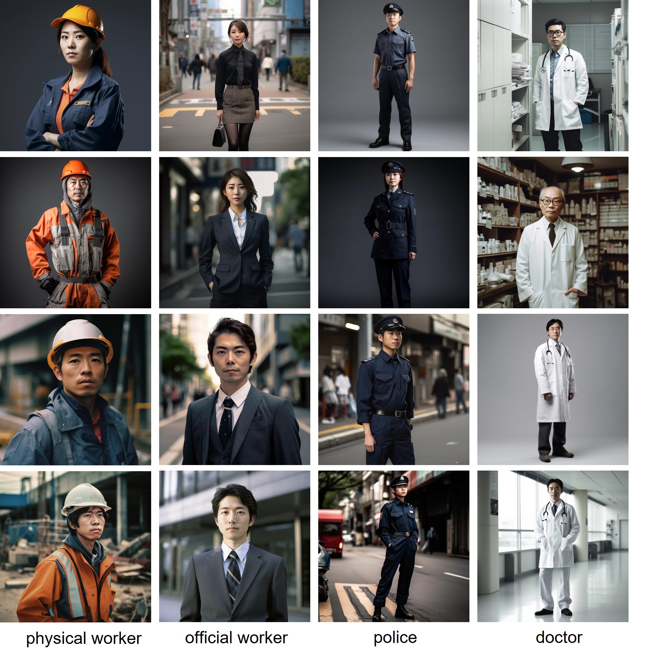
• Description of the JPOCC dataset creation using AI-generated images: The Japan Occupation Classification Challenge (JPOCC) dataset was created using AI-generated images to represent various occupations. This dataset is crucial for building an occupation classification model, as it provides a diverse range of images for training and evaluation. By using AI-generated images, we can ensure a large and varied dataset, which helps in improving the robustness and accuracy of the model.
• Categories included in the dataset (e.g., police, physical worker): The JPOCC dataset includes a variety of occupational categories such as police officers, physical workers, teachers, doctors, engineers, and many more. These categories are designed to cover a broad spectrum of professions, allowing the model to generalize well across different occupational groups.

Model Construction:

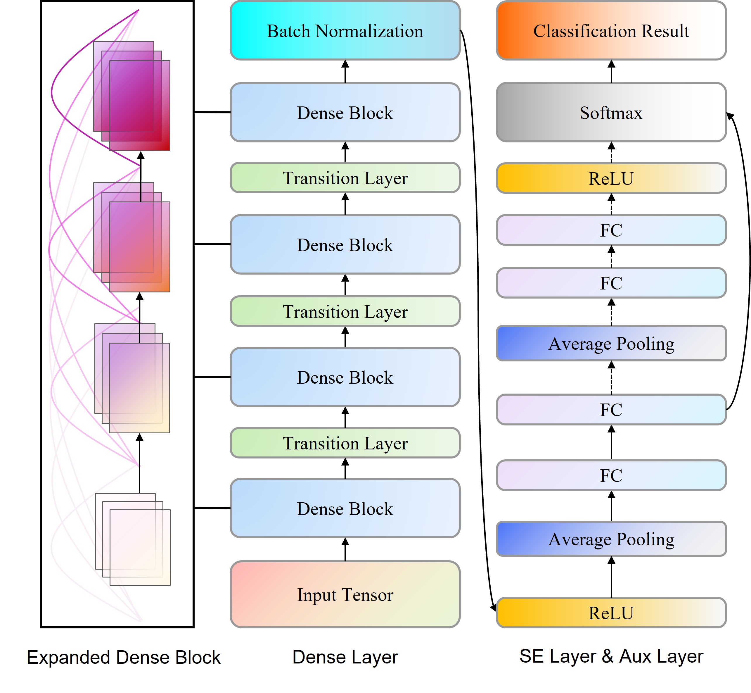
• Explanation of the DenseNet-161 architecture: DenseNet-161 is a deep convolutional neural network that connects each layer to every other layer in a feed-forward fashion. This architecture improves the flow of information and gradients throughout the network, making the model more efficient and easier to train.
• Integration of the SE module and auxiliary classifiers to enhance model performance: The Squeeze-and-Excitation (SE) module is integrated into the DenseNet-161 architecture to enhance its performance. The SE module improves the model’s ability to focus on important features by recalibrating channel-wise feature responses.
• Training process and use of the dataset for classification: The training process involves data preprocessing, model initialization, training with backpropagation, and evaluation. The JPOCC dataset is used to train the DenseNet-161 model with the SE module and auxiliary classifiers.

Here’s a concise code snippet illustrating this process:

import torch
import torch.nn as nn
import torch.optim as optim
from torchvision import datasets, transforms, models
from torch.utils.data import DataLoader

# Define the SE module
class SEBlock(nn.Module):
    def __init__(self, in_channels, reduction=16):
        super(SEBlock, self).__init__()
        self.fc1 = nn.Conv2d(in_channels, in_channels // reduction, kernel_size=1)
        self.fc2 = nn.Conv2d(in_channels // reduction, in_channels, kernel_size=1)
        self.sigmoid = nn.Sigmoid()

    def forward(self, x):
        w = nn.functional.adaptive_avg_pool2d(x, 1)
        w = self.fc1(w)
        w = nn.ReLU(inplace=True)(w)
        w = self.fc2(w)
        w = self.sigmoid(w)
        return x * w

# Define the model with SE module and auxiliary classifiers
class DenseNet161_SE(nn.Module):
    def __init__(self, num_classes=10):
        super(DenseNet161_SE, self).__init__()
        self.densenet = models.densenet161(pretrained=True)
        self.seblock = SEBlock(in_channels=2208)
        self.fc = nn.Linear(2208, num_classes)
        self.auxiliary_fc = nn.Linear(768, num_classes)

    def forward(self, x):
        features = self.densenet.features(x)
        features = self.seblock(features)
        out = nn.functional.relu(features, inplace=True)
        out = nn.functional.adaptive_avg_pool2d(out, (1, 1)).view(out.size(0), -1)
        aux_out = self.auxiliary_fc(features.view(features.size(0), -1))
        final_out = self.fc(out)
        return final_out, aux_out

# Define data transformations
transform = transforms.Compose([
    transforms.Resize(256),
    transforms.CenterCrop(224),
    transforms.ToTensor(),
    transforms.Normalize(mean=[0.485, 0.456, 0.406], std=[0.229, 0.224, 0.225]),
])

# Load the dataset
train_dataset = datasets.ImageFolder(root='path_to_train_data', transform=transform)
val_dataset = datasets.ImageFolder(root='path_to_val_data', transform=transform)

train_loader = DataLoader(train_dataset, batch_size=32, shuffle=True)
val_loader = DataLoader(val_dataset, batch_size=32, shuffle=False)

# Initialize the model, loss function, and optimizer
model = DenseNet161_SE(num_classes=len(train_dataset.classes)).cuda()
criterion = nn.CrossEntropyLoss()
optimizer = optim.Adam(model.parameters(), lr=0.001)

# Training loop
for epoch in range(num_epochs):
    model.train()
    running_loss = 0.0
    for inputs, labels in train_loader:
        inputs, labels = inputs.cuda(), labels.cuda()
        optimizer.zero_grad()
        outputs, aux_outputs = model(inputs)
        loss = criterion(outputs, labels) + 0.4 * criterion(aux_outputs, labels)
        loss.backward()
        optimizer.step()
        running_loss += loss.item()

    print(f"Epoch [{epoch+1}/{num_epochs}], Loss: {running_loss/len(train_loader)}")

    # Validation
    model.eval()
    val_loss = 0.0
    correct = 0
    total = 0
    with torch.no_grad():
        for inputs, labels in val_loader:
            inputs, labels = inputs.cuda(), labels.cuda()
            outputs, _ = model(inputs)
            loss = criterion(outputs, labels)
            val_loss += loss.item()
            _, predicted = torch.max(outputs.data, 1)
            total += labels.size(0)
            correct += (predicted == labels).sum().item()

    print(f"Validation Loss: {val_loss/len(val_loader)}, Accuracy: {100 * correct/total}%")

Explanation:

• SEBlock class: Defines the Squeeze-and-Excitation block, which recalibrates channel-wise feature responses.
• DenseNet161_SE class: Integrates the DenseNet-161 architecture with the SE block and auxiliary classifiers.
• Data Transformations: Preprocess the images with resizing, cropping, normalization, etc.
• Data Loading: Load the training and validation datasets.
• Training Loop: Train the model using backpropagation and evaluate it on the validation set.

By implementing this approach, we can effectively classify occupations based on images, providing valuable insights into consumer demographics and enabling more personalized and targeted marketing strategies. This comprehensive model construction and training process ensures high accuracy and robustness in occupation classification.

2. Product Status Control

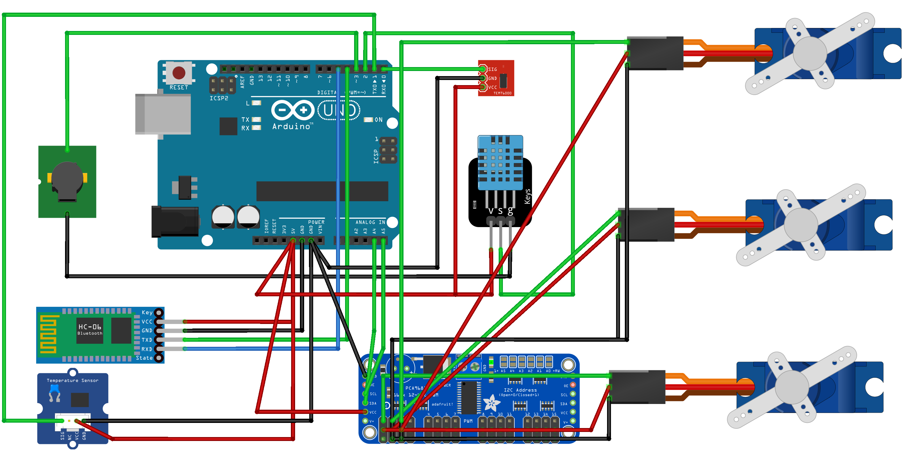
• 2.1 System Components:
  • Overview of the Arduino-based product status control system.
  • Description of the hardware components used (e.g., servo motors, sensors).
• 2.2 Algorithm:
  • Explanation of the algorithm used for product status monitoring and dispensing.
  • Details of the control system operation logic.

Algorithm Product Status Control Algorithm

Require: HC – 06, ServoDriver, DHT11, A0, A1, Buzzer

1. Initialize HC – 06, ServoDriver, DHT11, A0, A1, Buzzer
2. Set object count: O1 ← 10, O2 ← 10, O3 ← 10
3. while True do
4.     Read HC – 06 input into ComA; Read light sensor value from A0 into L; Read gas sensor value from A1 into G; Read humidity and temperature from DHT11 into H and T
5.     Compose and send data string; Activate Buzzer if G > 60 else deactivate Buzzer
6.     if ComA contains valid data then
7.         Parse age information into Old; Set Flag ← True
8.     end if
9.     if Old < 30 and Flag and O1 > 0 then
10.         Dispense object 1; Update O1 ← O1 – 1; Set Flag ← False
11.     else if 30 ≤ Old < 60 and Flag and O2 > 0 then
12.         Dispense object 2; Update O2 ← O2 – 1; Set Flag ← False
13.     else if Old ≥ 60 and Flag and O3 > 0 then
14.         Dispense object 3; Update O3 ← O3 – 1; Set Flag ← False
15.     end if
16. end while

• 2.3 Application:
  • Integration with a mobile app for real-time monitoring and control.
  • Description of communication between Arduino and the mobile application.

3. Experiment

• 3.1 Consumer Portrait Model Evaluation:
  • Dataset Preparation:
    • Steps for preprocessing the JPOCC dataset (e.g., resizing images, data augmentation).
    • Splitting the dataset into training, validation, and test sets.
  • Training Process:
    • Key parameters for training (e.g., batch size, weight decay, epochs).
    • Use of data augmentation techniques.
    • Introduction of the SE module and auxiliary classifiers during training.
  • Comparison with Other Models:
    • Evaluation metrics (e.g., accuracy, precision, recall, F1 score).
    • Comparison of the ASD model with other classifiers (e.g., SVM, KNN, CNN, ResNet).
• 3.2 Sentiment Analysis Model Application:
  • Selection of Products:
    • Criteria for selecting energy drinks for the experiment.
    • Creation of product cards with key information.
    • For official testing, we created “product cards” for the ten drinks based on the official product manuals, official advertising campaigns, and research reports from reputable third-party testing organizations. These product cards contain key information: 1. Drink name; 2. Manufacturer; 3. Main ingredients; 4. Efficacy; 5. Notes. Figure 6 displays the product cards for two drinks.
  • Consumer Reports:
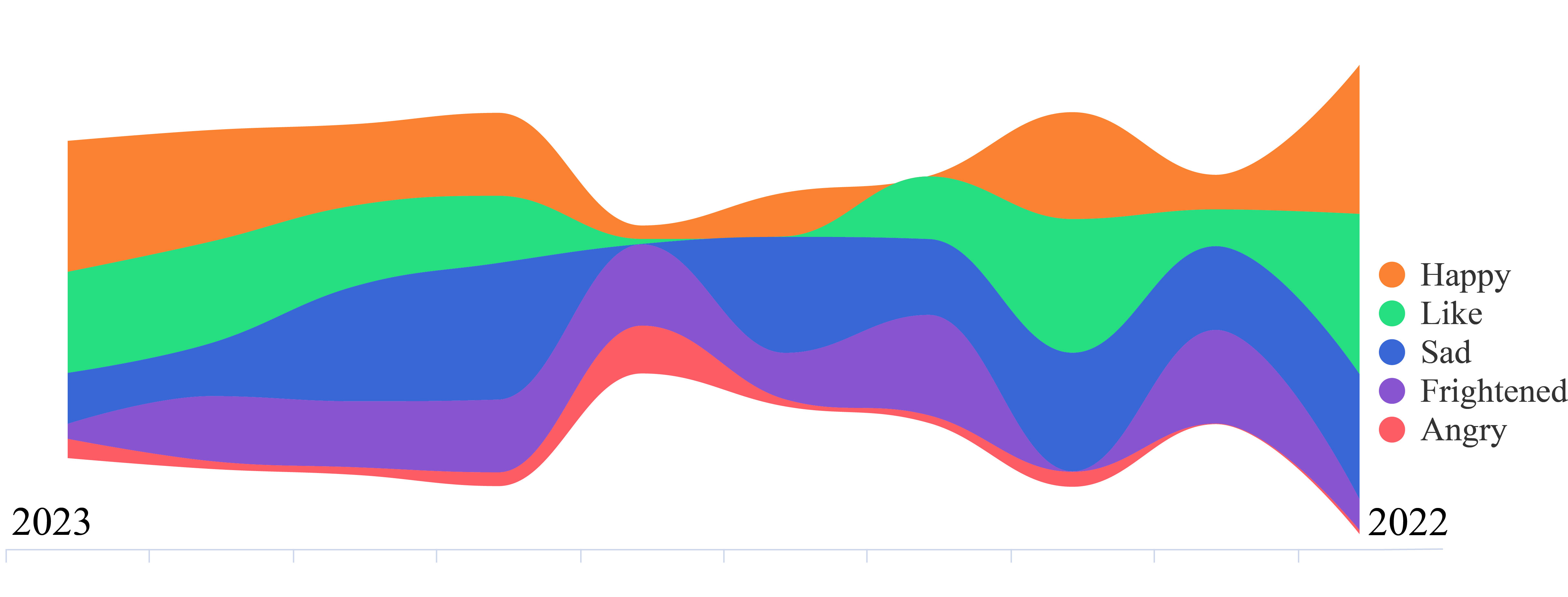
    • Collection and analysis of consumer reviews.
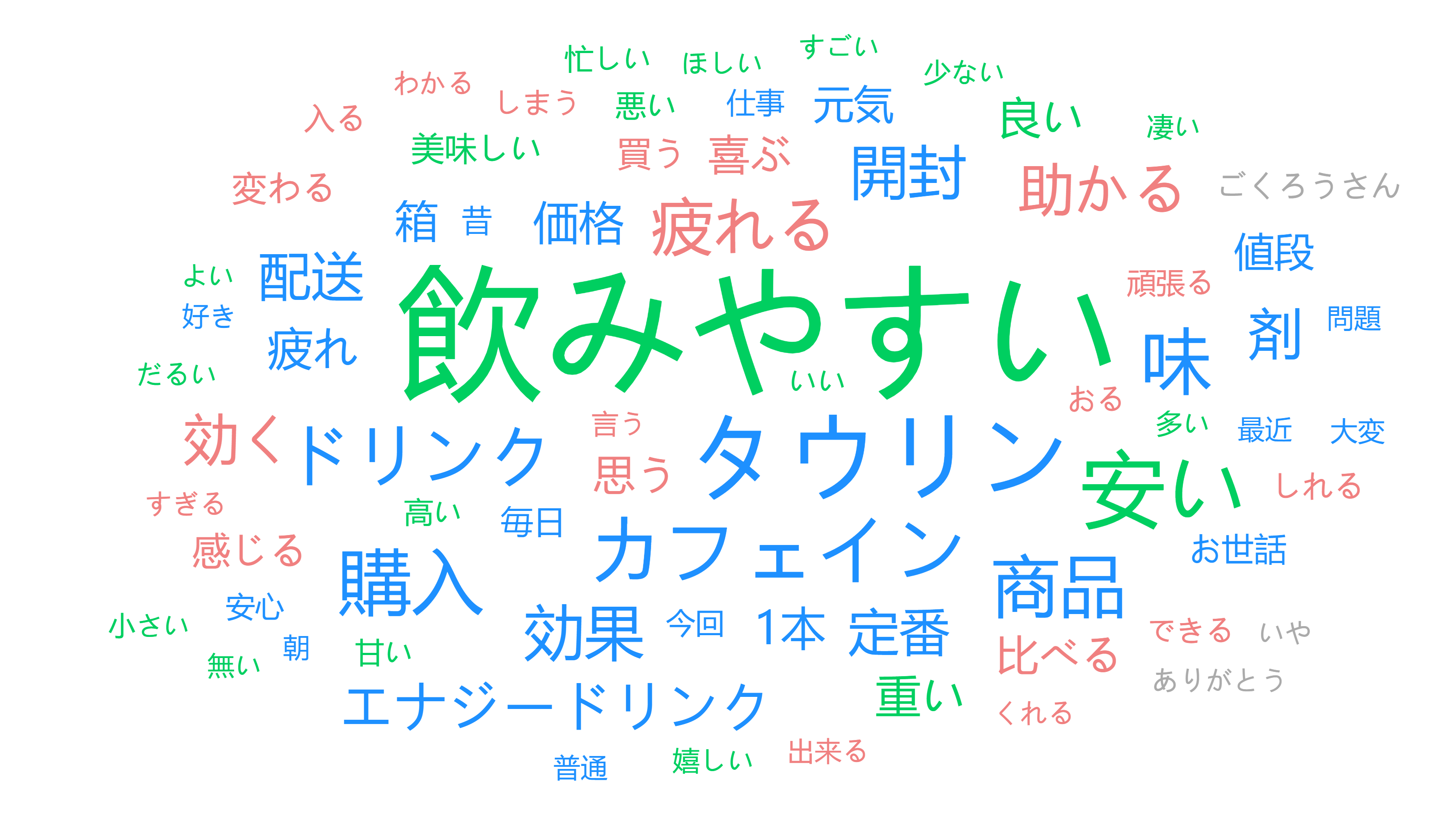
    • Use of word cloud visualizations and TF-IDF values for product tags.
  • Character Cards:
    • Creation of character cards for target audiences.
    • Attributes included in character cards (e.g., age, gender, behavior type).
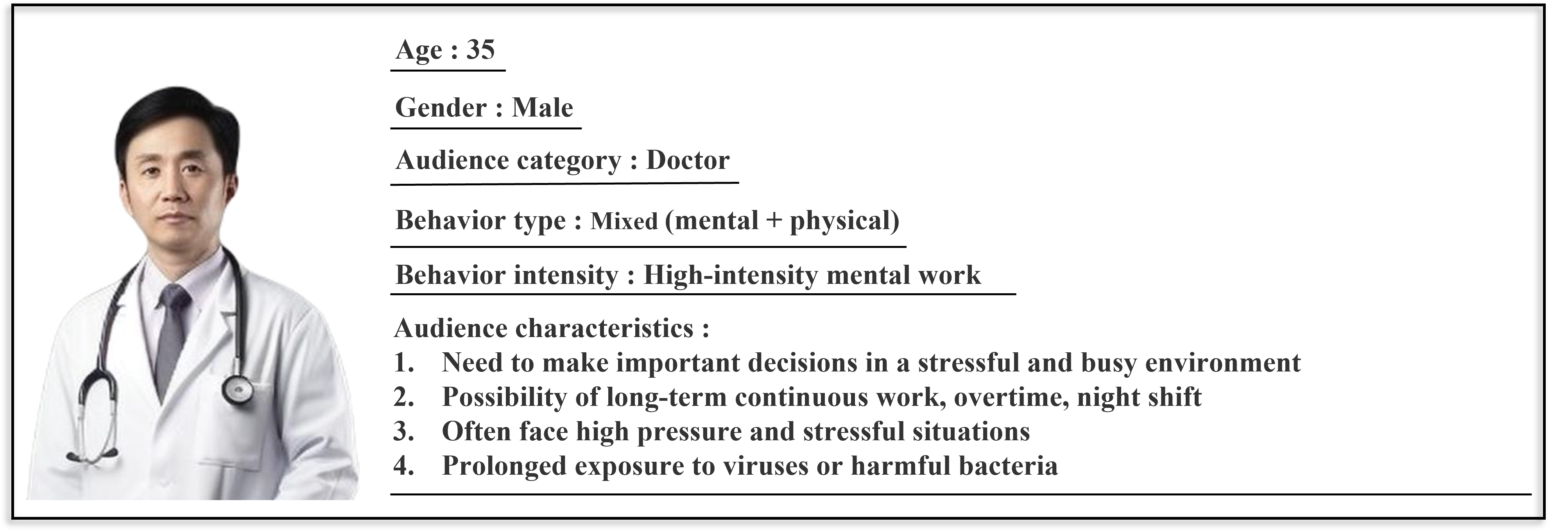
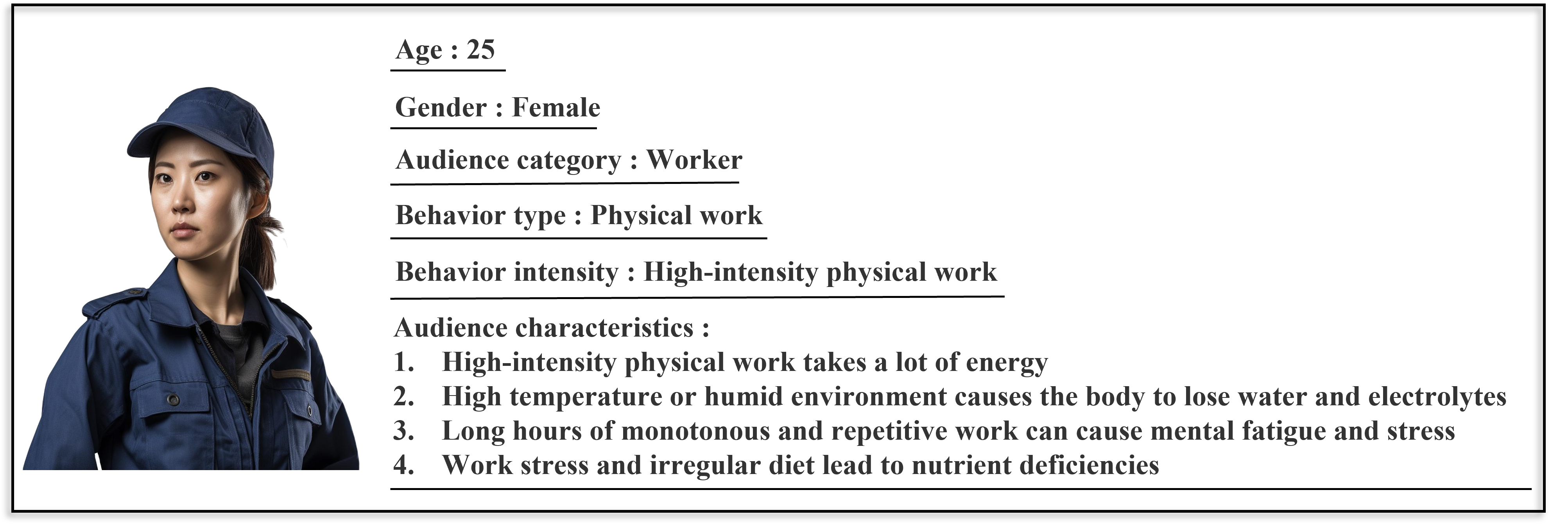
    • Besides product cards, we also created “character cards” for eight different target audiences using research and information from relevant science communication websites. These cards include: 1. Age; 2. Gender; 3. Audience category; 4. Behaviour type; 5. Behaviour intensity; 6. Audience characteristics.
  • Adaptability Analysis:
    • Inputting product and character card data into GPT-4 for semantic analysis.
    • Categorization of adaptability levels (e.g., perfect fit, general fit, no fit).
    • Presentation of adaptability results for different demographics.