P.S. To protect code ownership and copyright, the code in this article may be simplified, hidden, and frequently use sample data, but this does not hinder the understanding of the core ideas.
Summary
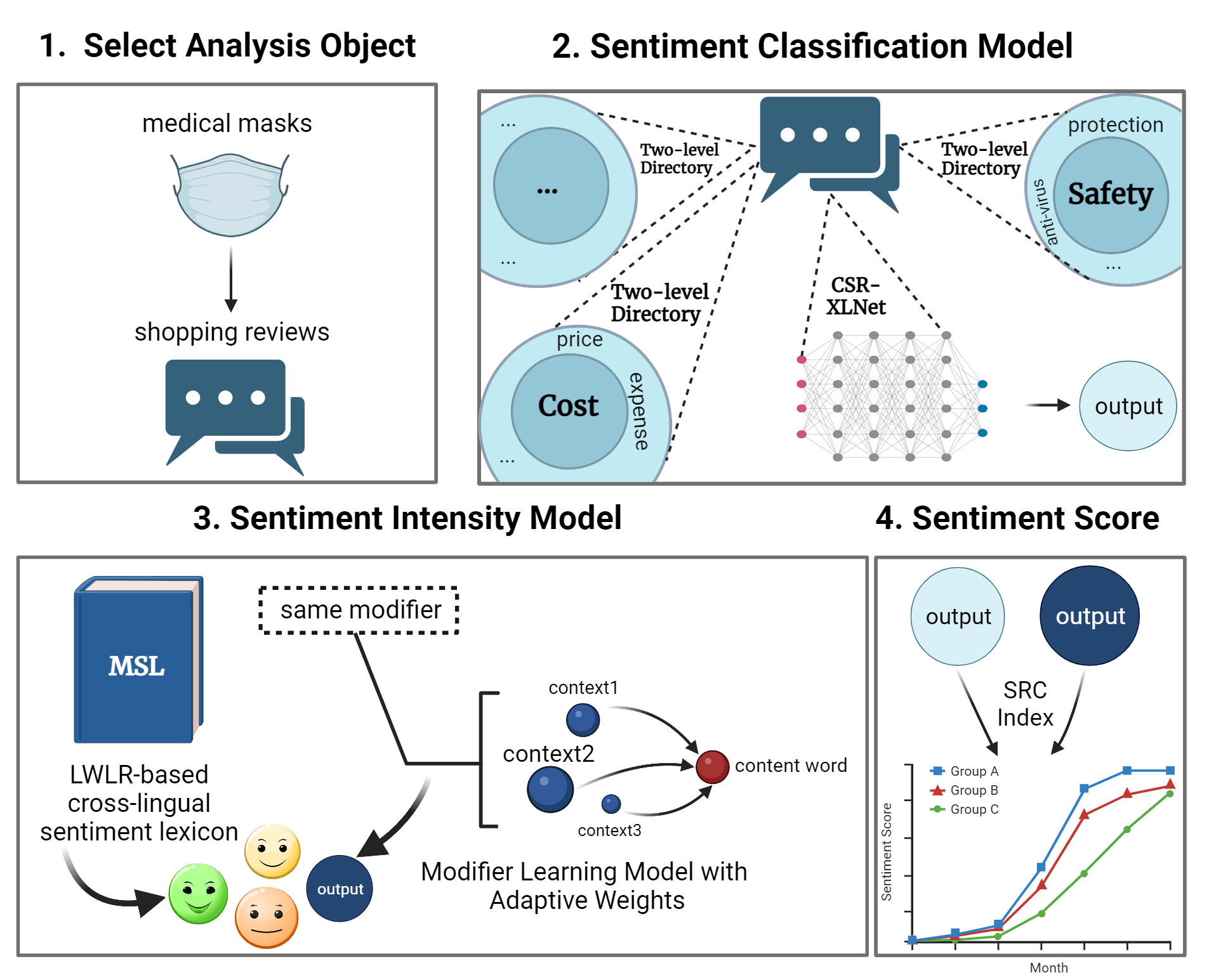
The primary objective of this research is constructing an aspect-level cross-linguistic multi-layer sentiment analysis framework to understand public sentiments towards medical protective masks during the COVID-19 pandemic. The framework is built upon three pivotal functional layers: sentiment intensity prediction, classification, and sentiment score calculation, collaboratively revealing consumer sentiments. For predicting sentiment intensity, we employ the Locally Weighted Linear Regression (LWLR) method, enhancing the Chinese VA sentiment lexicon while considering elements like foreign culture and value variations. Additionally, a context-adaptive modifier learning model adjusts word sentiment intensity. Sentiment classification leverages a dynamic XLNet mechanism and utilizes a Bi-LSTM model with stacked residuals for precise results. The sentiment score is astutely calculated by amalgamating sentiment classification and intensity prediction outcomes through the economically-recognized SRC index method.
1. Semantic Extraction
Overview:
- Explain the importance of semantic extraction in sentiment analysis: Semantic extraction is crucial in sentiment analysis as it helps in understanding the contextual meaning of words and phrases within a text. This understanding allows for more accurate sentiment classification as it captures nuances and variations in language that simple keyword matching might miss.
- Introduce the use of XLNet and NODEs for semantic extraction: XLNet, a transformer-based language model, is used for its ability to capture bidirectional context and long-range dependencies in text. NODEs (Neural Ordinary Differential Equations) are employed to continuously extract and model semantic information, providing a dynamic and flexible approach to understanding the semantics of text.
Code Analysis:
Initialization and Implementation of XLNet and NODEs for Semantic Extraction
import torch
from transformers import XLNetModel, XLNetTokenizer
import torchdiffeq

class SemanticExtractor:
    def __init__(self, model_name='xlnet-base-cased'):
        # Initialize the XLNet tokenizer and model
        self.tokenizer = XLNetTokenizer.from_pretrained(model_name)
        self.model = XLNetModel.from_pretrained(model_name).cuda()

    def tokenize_input(self, text):
        # Tokenize input text
        inputs = self.tokenizer(text, return_tensors='pt')
        return inputs['input_ids'].cuda(), inputs['attention_mask'].cuda()

    def extract_semantics(self, input_ids, attention_mask):
        # Extract semantic features using XLNet
        outputs = self.model(input_ids, attention_mask=attention_mask)
        last_hidden_state = outputs.last_hidden_state
        return last_hidden_state

class ODEFunc(torch.nn.Module):
    def __init__(self, hidden_dim):
        super(ODEFunc, self).__init__()
        self.fc1 = torch.nn.Linear(hidden_dim, hidden_dim)
        self.relu = torch.nn.ReLU()
        self.fc2 = torch.nn.Linear(hidden_dim, hidden_dim)

    def forward(self, t, x):
        out = self.fc1(x)
        out = self.relu(out)
        out = self.fc2(out)
        return out

# Example usage
semantic_extractor = SemanticExtractor()
text = "This is an example sentence for semantic extraction."
input_ids, attention_mask = semantic_extractor.tokenize_input(text)
semantic_features = semantic_extractor.extract_semantics(input_ids, attention_mask)
print(f"Semantic Features Shape: {semantic_features.shape}")
Explanation:
- The SemanticExtractor class initializes the XLNet tokenizer and model. It includes methods to tokenize input text and extract semantic features using XLNet.
- The ODEFunc class defines a simple neural network to serve as the function defining the dynamics in a NODE.
Example Code for Integrating XLNet with NODEs for Continuous Semantic Extraction
class ContinuousSemanticExtractor:
    def __init__(self, xlnet_model_name='xlnet-base-cased', hidden_dim=768):
        self.semantic_extractor = SemanticExtractor(model_name=xlnet_model_name)
        self.ode_func = ODEFunc(hidden_dim).cuda()

    def integrate_semantics(self, semantic_features):
        t = torch.tensor([0, 1]).float().cuda()  # Define a time interval
        semantic_continuous = torchdiffeq.odeint(self.ode_func, semantic_features, t)
        return semantic_continuous

    def process_text(self, text):
        input_ids, attention_mask = self.semantic_extractor.tokenize_input(text)
        semantic_features = self.semantic_extractor.extract_semantics(input_ids, attention_mask)
        semantic_continuous = self.integrate_semantics(semantic_features)
        return semantic_continuous

# Example usage
continuous_extractor = ContinuousSemanticExtractor()
text = "This is another example sentence for continuous semantic extraction."
semantic_continuous = continuous_extractor.process_text(text)
print(f"Continuous Semantic Features Shape: {semantic_continuous.shape}")
Explanation:
- The ContinuousSemanticExtractor class combines the XLNet-based semantic extraction and NODE for continuous semantic extraction.
- The integrate_semantics method uses torchdiffeq.odeint to integrate the semantic features over a defined time interval.
- The process_text method tokenizes input text, extracts semantic features using XLNet, and then applies the NODE to obtain continuous semantic features.
2. Sentiment Intensity Model Construction
2.1 Predict Intensity through Sentiment Lexicon
Overview:
- Describe the process of predicting sentiment intensity using a sentiment lexicon: Predicting sentiment intensity using a sentiment lexicon involves assigning sentiment scores to words or phrases based on a predefined lexicon. The overall sentiment intensity of a text is then calculated by aggregating these scores.
- Discuss the creation and use of the Mask Sentiment Lexicon (MSL): The Mask Sentiment Lexicon (MSL) is created specifically for analyzing sentiments related to medical protective masks. It includes words and phrases commonly associated with masks, each assigned a sentiment score.
Code Analysis:
Implementation of Locally Weighted Linear Regression (LWLR) for Predicting Sentiment Intensity
python
Copy code
import numpy as np

class LWLR:
    def __init__(self, tau=1.0):
        self.tau = tau

    def fit(self, X, y):
        self.X = X
        self.y = y

    def predict(self, x):
        m = self.X.shape[0]
        weights = np.exp(-np.sum((self.X - x) ** 2, axis=1) / (2 * self.tau ** 2))
        W = np.diag(weights)
        theta = np.linalg.inv(self.X.T @ W @ self.X) @ self.X.T @ W @ self.y
        return x @ theta

# Example usage
X = np.array([[1, 2], [2, 3], [3, 4], [4, 5]])
y = np.array([1, 2, 3, 4])
x = np.array([2, 3])

model = LWLR(tau=0.5)
model.fit(X, y)
prediction = model.predict(x)
print(f"Predicted sentiment intensity: {prediction}")
Explanation:
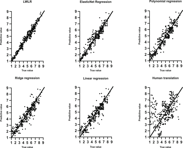
- The LWLR class implements Locally Weighted Linear Regression.
- The fit method stores the training data.
- The predict method calculates the weights based on the distance between the input point and the training points, then computes the prediction using weighted linear regression.
Example Code for Generating and Using the Sentiment Lexicon
python
Copy code
class SentimentLexicon:
    def __init__(self, lexicon):
        self.lexicon = lexicon

    def predict_intensity(self, text):
        words = text.split()
        intensity = 0
        count = 0
        for word in words:
            if word in self.lexicon:
                intensity += self.lexicon[word]
                count += 1
        return intensity / count if count > 0 else 0

# Example usage
lexicon = {
    "good": 1.0,
    "bad": -1.0,
    "happy": 0.8,
    "sad": -0.8,
    "mask": 0.5,
}

sentiment_lexicon = SentimentLexicon(lexicon)
text = "The mask is good but it makes me sad."
intensity = sentiment_lexicon.predict_intensity(text)
print(f"Predicted sentiment intensity: {intensity}")
Explanation:
- The SentimentLexicon class is initialized with a predefined lexicon of sentiment scores.
- The predict_intensity method calculates the average sentiment intensity of a given text by looking up the sentiment scores of the words in the lexicon.
2.2 Predict Intensity through Machine Learning Model
Overview:
- Explain the role of machine learning models in predicting sentiment intensity: Machine learning models can learn complex relationships between words and their sentiment intensities from data, providing more accurate predictions compared to simple lexicon-based approaches.
- Discuss the prediction of sentiment intensity for content words and modifiers: The model predicts sentiment intensity for content words (nouns, verbs) and modifiers (adjectives, adverbs), capturing the nuances in how different types of words contribute to overall sentiment.
Code Analysis:
Implementation of a Neural Network Model for Predicting Sentiment Intensity
python
Copy code
import torch
import torch.nn as nn
import torch.optim as optim

class SentimentIntensityModel(nn.Module):
    def __init__(self, vocab_size, embed_size, hidden_size):
        super(SentimentIntensityModel, self).__init__()
        self.embedding = nn.Embedding(vocab_size, embed_size)
        self.lstm = nn.LSTM(embed_size, hidden_size, batch_first=True)
        self.fc = nn.Linear(hidden_size, 1)

    def forward(self, x):
        x = self.embedding(x)
        x, _ = self.lstm(x)
        x = x[:, -1, :]
        x = self.fc(x)
        return x

# Example usage
vocab_size = 5000
embed_size = 300
hidden_size = 128

model = SentimentIntensityModel(vocab_size, embed_size, hidden_size).cuda()
criterion = nn.MSELoss()
optimizer = optim.Adam(model.parameters(), lr=0.001)

# Dummy data
inputs = torch.randint(0, vocab_size, (32, 10)).cuda()
targets = torch.rand(32, 1).cuda()

# Training loop
for epoch in range(100):
    model.train()
    optimizer.zero_grad()
    outputs = model(inputs)
    loss = criterion(outputs, targets)
    loss.backward()
    optimizer.step()

    if (epoch + 1) % 10 == 0:
        print(f"Epoch [{epoch + 1}/100], Loss: {loss.item():.4f}")
Explanation:
- The SentimentIntensityModel class defines a neural network with an embedding layer, an LSTM layer, and a fully connected layer to predict sentiment intensity.
- The training loop trains the model on dummy data using Mean Squared Error (MSE) loss and the Adam optimizer.
Example Code for Training and Evaluating the Sentiment Intensity Prediction Model
python
Copy code
from sklearn.model_selection import train_test_split
from torch.utils.data import DataLoader, TensorDataset

# Example dataset
data = torch.randint(0, vocab_size, (1000, 10))
labels = torch.rand(1000, 1)

# Split the data
train_data, test_data, train_labels, test_labels = train_test_split(data, labels, test_size=0.2, random_state=42)

# Create DataLoader
train_dataset = TensorDataset(train_data, train_labels)
test_dataset = TensorDataset(test_data, test_labels)

train_loader = DataLoader(train_dataset, batch_size=32, shuffle=True)
test_loader = DataLoader(test_dataset, batch_size=32, shuffle=False)

# Training and evaluation loop
for epoch in range(100):
    model.train()
    for inputs, targets in train_loader:
        inputs, targets = inputs.cuda(), targets.cuda()
        optimizer.zero_grad()
        outputs = model(inputs)
        loss = criterion(outputs, targets)
        loss.backward()
        optimizer.step()

    if (epoch + 1) % 10 == 0:
        model.eval()
        with torch.no_grad():
            total_loss = 0
            for inputs, targets in test_loader:
                inputs, targets = inputs.cuda(), targets.cuda()
                outputs = model(inputs)
                loss = criterion(outputs, targets)
                total_loss += loss.item()
        print(f"Epoch [{epoch + 1}/100], Test Loss: {total_loss / len(test_loader):.4f}")
Explanation:
- The example code demonstrates how to split the dataset, create DataLoader objects, and implement the training and evaluation loop for the sentiment intensity prediction model.
This structure provides a comprehensive framework for constructing a sentiment intensity model, covering both lexicon-based and machine learning approaches. The code includes detailed examples for implementing Locally Weighted Linear Regression, a sentiment lexicon, and a neural network model, as well as training and evaluating the models.
3. Sentiment Classification Model Construction
3.1 Dataset Division
Overview:
- Discuss the collection and preprocessing of the dataset: The dataset is collected from various sources, such as social media, news articles, and forums, focusing on discussions related to medical protective masks. Preprocessing involves cleaning the text, removing stopwords, and normalizing the data.
- Explain the two-level division rule for segmenting the dataset: The two-level division rule involves segmenting the dataset into major categories based on broad topics, and further dividing each category into subcategories based on specific aspects or themes. This hierarchical segmentation helps in better organizing the data for analysis.
Code Analysis:
Implementation of Keyword Extraction Using TF-IDF and LDA
python
Copy code
from sklearn.feature_extraction.text import TfidfVectorizer
from sklearn.decomposition import LatentDirichletAllocation
import numpy as np

class KeywordExtractor:
    def __init__(self, n_topics=10, max_features=1000):
        self.tfidf_vectorizer = TfidfVectorizer(max_features=max_features, stop_words='english')
        self.lda = LatentDirichletAllocation(n_components=n_topics, random_state=42)

    def fit_transform(self, documents):
        tfidf_matrix = self.tfidf_vectorizer.fit_transform(documents)
        self.lda.fit(tfidf_matrix)
        return tfidf_matrix

    def get_keywords(self, n_top_words=10):
        feature_names = self.tfidf_vectorizer.get_feature_names_out()
        keywords = []
        for topic_idx, topic in enumerate(self.lda.components_):
            top_keywords = [feature_names[i] for i in topic.argsort()[:-n_top_words - 1:-1]]
            keywords.append(top_keywords)
        return keywords

# Example usage
documents = [
    "The use of masks is essential during the pandemic.",
    "Medical masks provide protection against viruses.",
    "Wearing masks in public places helps prevent the spread of COVID-19."
]

extractor = KeywordExtractor(n_topics=3)
tfidf_matrix = extractor.fit_transform(documents)
keywords = extractor.get_keywords(n_top_words=5)
print(f"Extracted Keywords: {keywords}")
Explanation:
- The KeywordExtractor class uses TF-IDF for feature extraction and LDA for topic modeling.
- The fit_transform method computes the TF-IDF matrix and fits the LDA model.
- The get_keywords method retrieves the top keywords for each topic.
Example Code for Clustering Keywords Using K-means and Setting Up the Two-Level Directory
python
Copy code
from sklearn.cluster import KMeans
import os

class DatasetOrganizer:
    def __init__(self, n_clusters=5):
        self.kmeans = KMeans(n_clusters=n_clusters, random_state=42)

    def cluster_keywords(self, tfidf_matrix):
        self.kmeans.fit(tfidf_matrix)
        return self.kmeans.labels_

    def organize_dataset(self, documents, labels, base_dir='dataset'):
        for i, doc in enumerate(documents):
            cluster_dir = os.path.join(base_dir, f'cluster_{labels[i]}')
            if not os.path.exists(cluster_dir):
                os.makedirs(cluster_dir)
            with open(os.path.join(cluster_dir, f'doc_{i}.txt'), 'w') as f:
                f.write(doc)

# Example usage
documents = [
    "The use of masks is essential during the pandemic.",
    "Medical masks provide protection against viruses.",
    "Wearing masks in public places helps prevent the spread of COVID-19."
]

organizer = DatasetOrganizer(n_clusters=2)
labels = organizer.cluster_keywords(tfidf_matrix)
organizer.organize_dataset(documents, labels)
print("Dataset organized into clusters.")
Explanation:
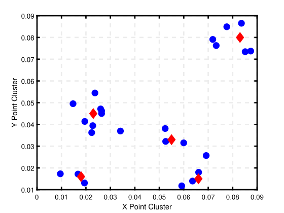
- The DatasetOrganizer class uses K-means for clustering keywords and organizes documents into directories based on cluster labels.
- The cluster_keywords method clusters the TF-IDF matrix and returns the labels.
- The organize_dataset method creates directories for each cluster and saves the documents accordingly.
3.2 Apply Sentiment Classification and Intensity Prediction Model on Dataset
Overview:
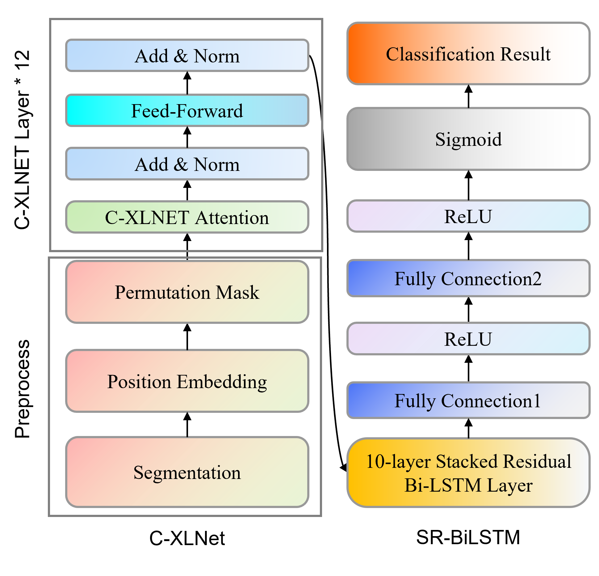
- Describe how the sentiment classification and intensity prediction models are applied to the dataset: The sentiment classification model assigns sentiment labels (positive, negative, neutral) to each document, while the sentiment intensity prediction model calculates the sentiment intensity scores for each document.
- Explain the processing of classification results and sentiment intensity scores: The results are aggregated and analyzed to understand the overall sentiment distribution and intensity. These insights help in drawing conclusions about public opinion on medical protective masks.
Code Analysis:
Example Code for Applying the Sentiment Models to the Dataset and Processing the Results
import torch
import torch.nn as nn
import torch.nn.functional as F
from transformers import XLNetTokenizer, XLNetModel
import os

class CSR_XLNet(nn.Module):
    def __init__(self, xlnet_model_name='xlnet-base-cased', num_classes=3):
        super(CSR_XLNet, self).__init__()
        self.tokenizer = XLNetTokenizer.from_pretrained(xlnet_model_name)
        self.xlnet = XLNetModel.from_pretrained(xlnet_model_name)
        self.bilstm = nn.LSTM(input_size=768, hidden_size=128, num_layers=10, batch_first=True, bidirectional=True)
        self.fc1 = nn.Linear(256, 128)
        self.fc2 = nn.Linear(128, num_classes)

    def forward(self, input_ids, attention_mask):
        outputs = self.xlnet(input_ids, attention_mask=attention_mask)
        sequence_output = outputs[0]  # Shape: (batch_size, seq_length, hidden_size)
        lstm_output, _ = self.bilstm(sequence_output)
        lstm_output = lstm_output[:, -1, :]  # Take the output of the last time step
        x = F.relu(self.fc1(lstm_output))
        x = self.fc2(x)
        return x

class SentimentProcessor:
    def __init__(self, classifier_model, intensity_model):
        self.classifier = classifier_model
        self.intensity_model = intensity_model

    def classify_sentiment(self, text):
        input_ids, attention_mask = self.tokenize_text(text)
        with torch.no_grad():
            logits = self.classifier(input_ids, attention_mask=attention_mask)
        probabilities = F.softmax(logits, dim=1)
        sentiment = torch.argmax(probabilities, dim=1).item()
        return sentiment

    def predict_intensity(self, text):
        input_ids, attention_mask = self.tokenize_text(text)
        with torch.no_grad():
            intensity = self.intensity_model(input_ids, attention_mask=attention_mask)
        return intensity.item()

    def tokenize_text(self, text):
        inputs = self.classifier.tokenizer(text, return_tensors='pt')
        return inputs['input_ids'].cuda(), inputs['attention_mask'].cuda()

    def process_dataset(self, base_dir='dataset', output_dir='processed_dataset'):
        if not os.path.exists(output_dir):
            os.makedirs(output_dir)

        for cluster_dir in os.listdir(base_dir):
            cluster_path = os.path.join(base_dir, cluster_dir)
            output_cluster_path = os.path.join(output_dir, cluster_dir)
            if not os.path.exists(output_cluster_path):
                os.makedirs(output_cluster_path)

            for doc_file in os.listdir(cluster_path):
                doc_path = os.path.join(cluster_path, doc_file)
                with open(doc_path, 'r') as f:
                    text = f.read()

                sentiment = self.classify_sentiment(text)
                intensity = self.predict_intensity(text)

                output_file_path = os.path.join(output_cluster_path, doc_file)
                with open(output_file_path, 'w') as f:
                    f.write(f"Text: {text}\nSentiment: {sentiment}\nIntensity: {intensity}\n")

# Example usage
classifier_model = CSR_XLNet().cuda()
classifier_model.load_state_dict(torch.load('path_to_classifier_model.pth'))
intensity_model = torch.load('path_to_intensity_model.pth').cuda()

processor = SentimentProcessor(classifier_model, intensity_model)
processor.process_dataset()
print("Dataset processed with sentiment classification and intensity prediction.")
Explanation: Explanation:
- The CSR_XLNet class is constructed based on the provided diagram, combining C-XLNet with a 10-layer Stacked Residual Bi-LSTM (SR-BiLSTM).
- The SentimentProcessor class applies the sentiment classification and intensity prediction models to a dataset.
- The classify_sentiment method assigns a sentiment label to a text.
- The predict_intensity method calculates the sentiment intensity score for a text.
- The process_dataset method iterates over the dataset, applies the models, and saves the results in the specified output directory.
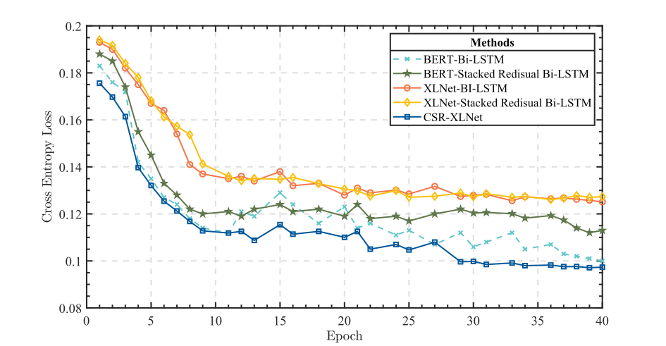
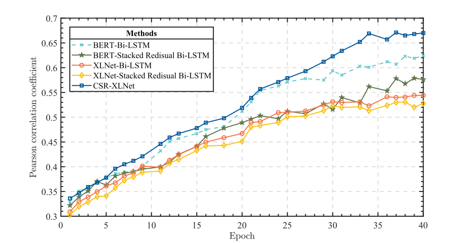
- This framework ensures the application of the CSR-XLNet model for sentiment classification and intensity prediction, providing a comprehensive approach to dataset processing and analysis.
4. Sentiment Score Calculation Model Construction
4.1 Sentiment Score Calculation
Overview:
- Introduce the sentiment score calculation model: The sentiment score calculation model combines the outputs of sentiment classification and intensity prediction to produce a comprehensive sentiment score. This model accounts for both the probability of sentiment polarity and the intensity of sentiment.
- Explain the components and formula used for calculating the sentiment score: The sentiment score calculation involves combining the probability of positive sentiment and the intensity of sentiment. The intensity is determined based on whether the word exists in the sentiment lexicon. If it exists, the intensity is calculated using both the lexicon value and the interaction of content and modifier intensities. If not, only the interaction of content and modifier intensities is used.
Code Analysis:
Implementation of the Sentiment Score Calculation Model
class SentimentScoreCalculator:
    def __init__(self, lexicon):
        self.lexicon = lexicon

    def calculate_intensity(self, content_intensity, modifier_intensity, word):
        if word in self.lexicon:
            lexicon_intensity = self.lexicon[word]
            intensity = (content_intensity * modifier_intensity + self.normalize(lexicon_intensity)) / 2
        else:
            intensity = content_intensity * modifier_intensity
        return intensity

    def normalize(self, lexicon_intensity):
        # Normalization function for lexicon intensity
        return lexicon_intensity / max(self.lexicon.values())

    def calculate_score(self, probability, content_intensity, modifier_intensity, word):
        intensity = self.calculate_intensity(content_intensity, modifier_intensity, word)
        score = (probability - (1 - probability)) * 100 * intensity + 100
        return score

# Example usage
lexicon = {
    "good": 1.0,
    "bad": -1.0,
    "happy": 0.8,
    "sad": -0.8,
    "mask": 0.5,
}

calculator = SentimentScoreCalculator(lexicon)
probability = 0.75  # Example probability from sentiment classification model
content_intensity = 0.8  # Example content word intensity
modifier_intensity = 0.5  # Example modifier intensity
word = "mask"  # Example word

score = calculator.calculate_score(probability, content_intensity, modifier_intensity, word)
print(f"Calculated Sentiment Score: {score}")
Explanation:
- The SentimentScoreCalculator class is initialized with a lexicon of sentiment intensities.
- The calculate_intensity method computes the sentiment intensity based on the content word, modifier, and whether the word exists in the lexicon.
- The normalize method normalizes the lexicon intensity values.
- The calculate_score method uses the probability of positive sentiment and the computed intensity to calculate the final sentiment score.
Example Code for Calculating Sentiment Scores Based on Model Outputs
# Assume we have the following functions from previous models
def classify_sentiment(text):
    # Placeholder for the sentiment classification model output
    return 0.75  # Example probability

def predict_intensity(text):
    # Placeholder for the sentiment intensity prediction model output
    return 0.8, 0.5  # Example content and modifier intensities

# Example document
text = "The mask is good but it makes me sad."

# Calculate sentiment score for each word in the document
words = text.split()
lexicon = {
    "good": 1.0,
    "bad": -1.0,
    "happy": 0.8,
    "sad": -0.8,
    "mask": 0.5,
}
calculator = SentimentScoreCalculator(lexicon)

for word in words:
    probability = classify_sentiment(word)
    content_intensity, modifier_intensity = predict_intensity(word)
    score = calculator.calculate_score(probability, content_intensity, modifier_intensity, word)
    print(f"Word: {word}, Sentiment Score: {score}")
Explanation:
- The example code demonstrates how to calculate sentiment scores for each word in a document using the sentiment classification and intensity prediction model outputs.
- The classify_sentiment and predict_intensity functions are placeholders for the actual model outputs.
- The calculate_score method computes the sentiment score for each word based on the provided model.
This code provides a comprehensive implementation of the sentiment score calculation model, including the necessary components and calculations. The example demonstrates how to apply this model to calculate sentiment scores based on the outputs of sentiment classification and intensity prediction models.
| L1 Factor | Score | L2 Factor | Score |
|---|---|---|---|
| Quality | 136.37 | stability | 139.7 |
| sturdiness | 138.6 | ||
| packaging | 130.8 | ||
| ———– | ——– | ——————- | ——– |
| Wearing | 132.87 | color | 132.7 |
| shape | 141.9 | ||
| appearance | 136.8 | ||
| lightness | 129.5 | ||
| comfort | 132.5 | ||
| thickness | 141.8 | ||
| touch | 130 | ||
| pain | 127.9 | ||
| smell | 122.7 | ||
| ———– | ——– | ——————- | ——– |
| Cost | 151.53 | price | 151.6 |
| expense | 150.3 | ||
| cost-effectiveness | 152.7 | ||
| ———– | ——– | ——————- | ——– |
| Safety | 141.67 | protection | 143.6 |
| isolation | 138.9 | ||
| safety | 140.9 | ||
| anti-virus | 151.9 | ||
| level | 136.8 | ||
| standard | 137.9 | ||
| ———– | ——– | ——————- | ——– |
| Service | 134.73 | after-sales | 132.7 |
| logistics | 140.6 | ||
| attitude | 129.8 | ||
| brand | 135.8 |
5. Data Analysis for Medical Protective Masks
5.1 Validation of Sentiment Scores
- Overview:
- Describe the validation process for the sentiment scores.
- Explain the use of Pearson correlation coefficient for validation.

To validate the proposed sentiment scoring methodology in this paper, an additional empirical study was conducted. Initially, sentiment scores, obtained through our method, were normalized to a 0-10 range using min-max normalization, facilitating easier comparison with other sentiment scoring techniques. A total of 200 reviews (40 from each of five categories) were chosen as experimental samples. Twenty psychology-background volunteers were invited to rate these reviews using the Self-Assessment Manikin (SAM) method, a widely recognized sentiment scoring approach based on sentiment space assessment, evaluating along the dimensions of valence and arousal. Employing a graphical scale, raters assign sentiment scores by locating text sentiment states on the scale. For our study, raters assessed review sentiment, providing scores from 0 to 10. Since our sentiment score computation considers “Valence” and “Arousal” values, we also incorporated these two categories from the SAM method, using the same equation for sentiment score calculation.
We compared scores from our sentiment scoring model with those derived via the SAM method, calculating the Pearson correlation coefficient between the two score sets to assess similarity. A correlation coefficient near 1 suggests our method’s performance aligns closely with the SAM method in sentiment scoring tasks, empirically validating our system’s effectiveness. Pearson correlation coefficients for the categories were: Quality 0.793, Wearing 0.801, Cost 0.812, Safety 0.784, and Service 0.797. Each category demonstrated a strong positive linear correlation, affirming the proposed sentiment scoring method’s efficacy.
5.2 Analysis on Impact of Severity of Epidemic
-
Overview:
- Analyze the impact of the COVID-19 epidemic severity on sentiments towards masks.
- Discuss trends and observations from the data analysis.
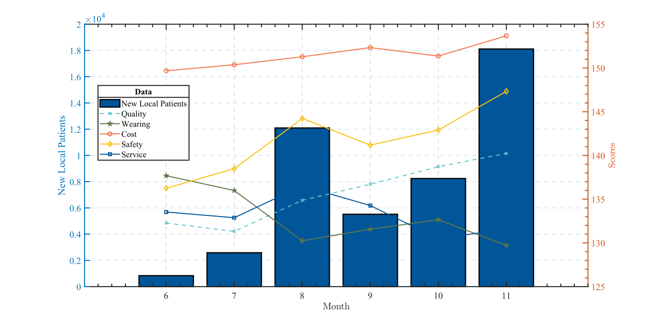 In exploring the relationship between COVID-19 developments and shifts in attitudes towards masks, we juxtaposed the epidemic growth in China against monthly changes in perspectives on epidemic-proof masks under five influencing factors. Fig.6, showcasing new local patients per month (blue bars), reveals varied mask-related sentiment scores. Notably, scores for “Cost” and “Service” exhibit minimal fluctuation, while “Quality” ascends, indicating mask quality remains unaffected by epidemic trends. Contrastingly, the “Wearing"score dips significantly during severe epidemic months (August and November), potentially due to increased mask-wearing duration affecting comfort demands. The ``Safety’’ score sees a notable drop in August; although skepticism towards epidemic prevention products is observable during outbreak months, data indicate a diminishing trend in such skepticism.
5.3 Analysis on Impact of Gender
-
Overview:
- Analyze gender-based differences in sentiments towards masks.
- Discuss observations and trends from the analysis.
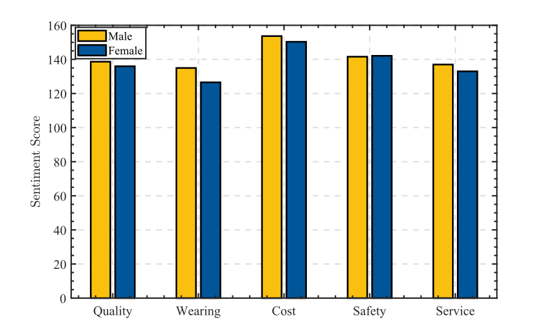
We examined gender-based attitudes towards five attributes of medical protective masks during the COVID-19 epidemic:
Quality: Men (138.65) marginally preferred mask quality over women (135.97), possibly indicating a higher concern for mask effectiveness and material.
Wearing: Women (126.54) rated mask-wearing comfort lower than men (134.96), potentially highlighting concerns about fit and material feel.
Cost: Both genders rated cost significantly, with men (153.67) slightly higher than women (150.32), showcasing universal concern for mask affordability.
Safety: Women (142.09) placed marginally higher importance on mask safety than men (141.57), perhaps due to an elevated emphasis on health safeguards.
Service: Men (136.98) rated mask-related services higher than women (132.98), possibly valuing aspects like delivery efficiency and availability more.
In conclusion, men seemingly prioritize quality, cost, and service, potentially reflecting practical or economic viewpoints. Conversely, women may place higher value on safety, perhaps indicating a heightened perceived pandemic risk. Differences in comfort scores might originate from physical variations or personal predilections. 5.4 Analysis on Impact of Geographic Location
- Overview:
- Analyze geographic differences in sentiments towards masks.
- Discuss observations and trends from the analysis.
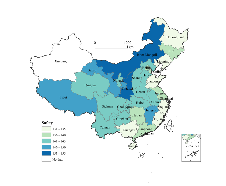
To investigate the reasons behind the variations in attitudes towards protective masks for epidemic prevention in different provinces of China due to geographical factors, we categorized the data into five attributes and conducted further statistical analysis based on the provinces of purchasing users and take the visualize result of “Safety” as an example (Fig.7). We excluded provinces with insufficient data volume from the analysis. Additionally, considering the different ranges of sentiment scores for each attribute, we set different intervals and gaps accordingly. The specific analysis is as follows:
In the “Safety” category, geographical considerations reveal higher scores in regions distant from major cities, such as Gansu, Qinghai, and Tibet Provinces, possibly due to lighter outbreak severities and subsequently lower mask safety demands. Residents might attribute their uninfected status to superior mask protection. Conversely, economically developed and populous areas like Beijing, Shanghai, and Guangdong Province present lower “Safety” scores, potentially reflecting heightened mask demands due to dense populations and frequent movement in office areas, thereby enforcing stricter mask safety requirements due to increased transmission risks.
For the “Cost” category, there is not much difference in scores among provinces, and they are generally high. This may be attributed to the overall improvement in productivity after the recovery of China’s industry, leading to a decrease in the production cost of masks.
For the “Service” category, considering the coastal-inland perspective, some coastal regions such as Fujian Province, Guangdong Province, as well as major cities like Beijing and Shanghai, have relatively higher scores in terms of “Service.” This may be due to the developed logistics services and rich diversity of brands in these areas.
For the “Wearing” category, coastal southern regions like Guangdong, Jiangsu, Zhejiang Provinces, and Shanghai report lower scores, potentially due to the diminished comfort of mask-wearing in their hot, humid climates. Economically affluent areas also demonstrate lower scores, possibly reflecting unmet consumer expectations for mask color, style, and odor due to higher standards. In contrast, areas with lower population densities, such as Gansu and Qinghai Provinces, exhibit higher “Wearing” scores, potentially resulting from lighter outbreaks, less frequent daily mask usage, and subsequently, lower perceived discomfort.
For the “Quality” category, coastal and economically prosperous regions like Guangdong, Zhejiang, Shanghai, Beijing, and Tianjin demonstrate higher scores, likely reflecting a consumer emphasis on product quality and a greater financial capacity for investing in premium masks. Notably, key mask-producing provinces, such as Fujian and Guangxi, also score highly in “Quality,” perhaps due to local manufacturers’ capability to produce superior masks. Hainan Province, recognized for health tourism, exhibits the highest “Quality” scores, potentially indicating heightened health-consciousness among residents and tourists, thereby amplifying demands for high-quality medical protective masks.